9.4 Usage
Quevedo is freely available on the Python Package Index (PyPI1) so the latest version can be
installed with the command python3 -m pip install quevedo. Source code is
available on GitHub2 under the Open Software License
3.03 and documentation is also
maintained using GitHub Pages4.
To build a dataset, we need a collection of images to annotate. We can then use the command line to create the dataset, configure it, and add the images to the relevant subset:
[path/to]$ python3 -m pip install quevedo
[path/to]$ quevedo -D dataset create
[path/to]$ cd dataset
[path/to/dataset]$ quevedo add_images -i source_image_directory -g trianglesAt this point, we will want to annotate the images. The first step is to decide on an annotation schema, an array of tags to give to logograms and graphemes, and the metadata schema, additional data which we will want to store about each file. This is configured in the dataset configuration file, which is in TOML format so easily editable with a text editor. An example configuration could be the following:
title = "Example dataset"

description = """
    This dataset is an imaginary example
    for how to use Quevedo. Annotations
    would be similar to those in vector
    graphics format such as SVG.
"""

tag_schema = [ "shape", "fill", "stroke" ]
meta_tags = [ "filename", "meaning" ]
...With this, the web interface can be launched, useful for both visualization of the source images and annotation of their meaning:
[path/to/dataset]$ quevedo web --host 'localhost' --port 8080Once the data have been annotated, the dataset can be accessed from user code to compute corpus statistics, perform user processing, or train machine learning algorithms. In the following example, we find the most common colors used in our imaginary dataset:
from collections import Counter
from quevedo import Dataset

colors = Counter()
ds = Dataset('path/to/dataset')

for a in ds.get_annotations():
    fill = a.tags['fill']
    stroke = a.tags['stroke']
    colors[fill] += 1
    colors[stroke] += 1

print(colors.most_common(5))To use the machine learning functionality provided with Quevedo, first we have to configure the networks and pipelines in the dataset configuration file:
[network.monochrome]
subject = "Classify black and white shapes"
task = "classify"
tag = [ "shape" ]
subsets = [ "squares", "triangles",
            "circles", "other" ]

[network.monochrome.filter]
criterion = "fill"
include = [ "black", "white" ]
# With this filter, only graphemes with a
# 'fill' tag of black or white will be
# used for training. This lets us have
# different networks for different tasks.With the network configured, we can then use the command line to
train it. This will take a bit of time, and at the end the network
weights will be stored in the network/monochrome
directory. These weights can be used to predict the “shape” tag of new
data, and we can do a basic test of its accuracy on our own data:
[p/t/dataset]$ quevedo -N monochrome train
Neural network 'monochrome' trained

[p/t/dataset]$ quevedo -N monochrome test
Annotations tested: 136
{
    "overall": 0.9632352941176471,
    "det_acc": 1.0,
    "cls_acc": 0.9632352941176471
}This is a basic introduction to Quevedo usage, and more detailed
documentation can be found online at https://agarsev.github.io/quevedo/latest/. The
command line interface can also list the available commands and
parameters with the command quevedo --help5.
In the next section we will give a brief overview of our own
dataset and research using Quevedo, including an example of the web
annotation. This dataset can be used to follow along with the
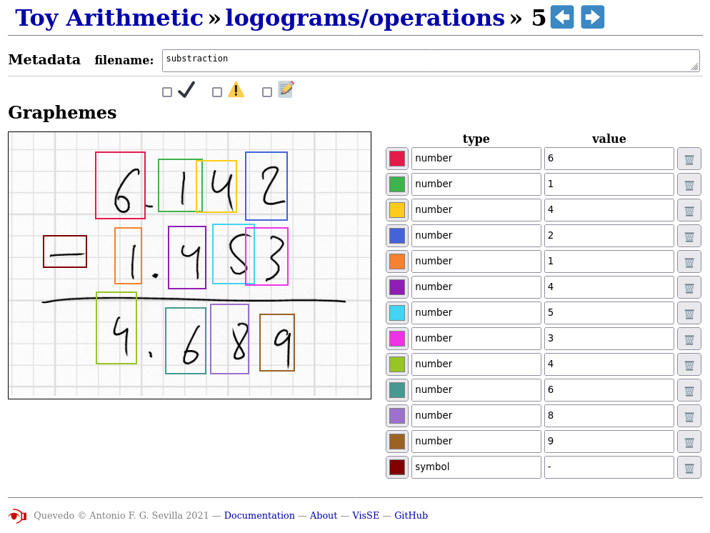
explanations in this section or on the online documentation. A simpler
example dataset is also provided with the Quevedo source code, and can
be found in the examples/toy_arithmetic directory. This
dataset also serves as an example of the how Quevedo can be used for
the annotation of different graphical languages, as it contains
examples of elementary arithmetic operations —additions,
substractions, etc., performed visually, as would be performed by
students. An example can be seen in Figure
9.4.
If the source code of Quevedo is downloaded, the latest development
features can be tested. For this, we recommend using
Poetry6, a python environment and
dependency manager. For example, we could clone the source code
repository and use Poetry to install dependencies,
allowing us to examine the example “toy arithmetic” dataset using the
web annotation interface. This would give a result similar to Figure
9.4, accessible using our own local browser. The following
sequence of commands, adapted to our own environment, could be used to
this end:
[~]$ git clone https://github.com/agarsev/quevedo
[~]$ cd quevedo
[quevedo]$ poetry install --extras "web"
[quevedo]$ cd examples/toy_arithmetic
[toy_arithmetic]$ poetry run quevedo info
[toy_arithmetic]$ poetry run quevedo web