7.1 Introduction

SignWriting is a writing system for sign languages (Sutton y Frost 2008). It uses the graphical possibilities of the bidimensional page to encode the visual characteristics of movement and space used in sign languages, so it is very different to other writing systems, especially in its non-linear nature.

The VisSE corpus is a collection of SignWriting instances, annotated graphically and semantically to capture all the meaning, both conventional and visual, of SignWriting. The samples are all handwritten, and codify signs or parts of signs from Spanish Sign Language. The samples were collected by Dr. José María Lahoz-Bengoechea during a span of years while learning Spanish Sign Language at Universidad Complutense de Madrid, and cover a wide range of vocabulary. However, since they were originally a tool for his private study and not for research, there may be minor errors and inconsistencies in the transcription. They should not be viewed as a collection of Spanish Sign Language Signs, but rather as a collection of SignWriting examples. Nonetheless, a tentative “gloss” (in Spanish) is included for most signs.

Due to the special nature of SignWriting, a tailored annotation schema is needed for its proper codification, and this is reflected both in the digital format of the corpus and in the logical structure of the annotations. This document is a guide for the later as well as a full and normative specification of it. The logical structure and possible values for the annotations are given, as well as some motivation or explanations when needed. For more detail on this, please see our forthcoming article “Building the VisSE corpus of Spanish SignWriting”.

It is not within the scope of this document to explain SignWriting. Interested readers can see the excellent and extensive documentation available online at https://signwriting.org/.

7.1.1 About examples

In this document, glyphs from the official Sutton SignWriting digital fonts are used to present examples for the different graphemes. This is done for two main reasons. On one hand, it is useful to present a “standard” and abstract example in each case and not choose any actual handwritten grapheme from the corpus as a “better” example. On the other hand, it may help users knowledgeable of SignWriting understand the schema even if some of the handwriting in the corpus is inconsistent or non standard.

It does not mean that only graphemes identical to the digital glyph will be tagged as such. SignWriting is very complicated, and there are variations available for many of its symbols. Additionally, handwriting tends to be less rigid than digital fonts, so variation is to be expected. Finally, some graphemes which are different symbols in the SignWriting specification have been tagged with the same label in this corpus. This is a conscious decision based on the phonology and the meaning of the graphemes in use in Spanish Sign Language, rather than the accurate and detailed phonetic description that SignWriting provides.

7.1.2 Annotation schema

SignWriting transcriptions are arrangements of symbols in a 2D space that represent the configuration of the hands, their orientation and movement, and other relevant features of signs in Sign Language. Each transcription can represent a single sign, or part of it. We call each independent arrangement of symbols a “logogram”, and we call each of the different symbols or graphical components a “grapheme”.

Graphemes have internal structure, both in their graphical properties (strokes, fill) and in their presentation (rotation, reflection). We encode these properties in a set of tags for each grapheme, a mapping of feature names to feature values that stores their meaning ‘in isolation’.

However, the meaning of each grapheme is not only determined by its graphical properties, but also by its position relative to the other graphemes in the logogram. This is codified for each grapheme with a ‘bounding box’, a square region within the logogram within which the grapheme can be found.

7.1.3 Grapheme tags

Not all classes of grapheme require the same number of features to annotate them. For this reason, graphemes are first roughly classified into six groups: HEAD, DIAC, HAND, ARRO, STEM and ARC. This is stored in the CLASS feature, common to all graphemes in the corpus. A more detailed classification of graphemes is then stored in the SHAPE feature, which is also common to all graphemes. The CLASS+SHAPE combination establishes the full ‘lexical’ meaning of the grapheme, but some grapheme CLASSes can have additional VAR, ROT and REF features which encode the rest of its ‘spatial’ meaning.

Each different CLASS in the corpus has a section in this guide, explaining the possible values of SHAPE, as well as any further tags needed to annotate them. In the case of HANDs, due to their complexity, a full chapter is dedicated to their annotation.

7.1.4 Bounding boxes

The location of each grapheme within the logogram is stored alongside its tags in the ‘bounding box’ attribute. This is a 4-tuple of floating point numbers, in the format \((cx, cy, w, h)\). \((cx, cy)\) are the coordinates of the center of the box relative to the logogram. The coordinates of the logogram go from \(0\) to \(1\), \((0, 0)\) being the top left corner, and \((1, 1)\) the bottom right one. \((w, h)\) are the width and height of the grapheme region, again relative to the width and height of the logogram (so ranging from \(0\) to \(1\)).

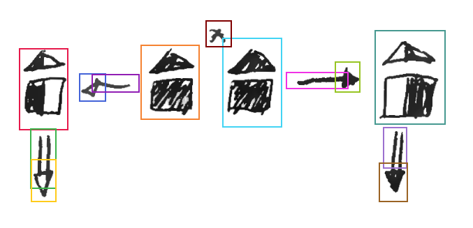
To visualize and create bounding boxes, a graphical tool is needed. Quevedo web interface provides such a tool, and shows the boxes as in Figure 7.1. Boxes should cover the full graphical extent of the grapheme, preferably with some padding around it. The exact location of the boxes is not important, but rather the general relative colocation of graphemes, as well as the full area covered by the grapheme’s symbol.

7.1.5 Programmatic access

This corpus is formatted as a Quevedo dataset, so the easier way to access the annotations is using the Quevedo library or command line tool. Since annotations have an important graphical component, Quevedo’s web interface can be especially useful in their visualization. To install Quevedo with the web interface, the command pip install quevedo[web] can be used in any system with python and pip installed.

Nonetheless, the annotations are stored in an open and standard format, so they can also be manually inspected or consumed by other tools.

7.1.6 Format on disk

Logograms in the corpus are stored in the logograms directory. They are split into subsets according to when they were collected, but subset structure is more organizational than semantically relevant. In each subset directory, logograms/A1_1 for example, logograms are sequentially numbered starting from the number 1.

Each logogram instance in the corpus consists of two files. First, the source image, with file extension .png, and then the annotation itself, with the same name but extension .json. For example, the annotation data corresponding to image logograms/A1_1/1.png is in file logograms/A1_1/1.json.

The json annotation file is a dictionary of attributes. It has a graphemes key, an array of the different graphemes found in the logogram, each of them having a box key with the bounding box coordinates (an array) and a tags key (a dictionary).

7.1.7 Other corpus objects

Inside the corpus root directory there are a number of other directories not mentioned above. The graphemes directory stores isolated graphemes samples. There are currently no such samples in the corpus, but they can be automatically extracted from the logograms. The networks directory stores the weights for neural networks trained with the corpus data, and useful code for processing the dataset can be found in the scripts directory. For more information on the dataset structure, please refer to Quevedo’s documentation at https://agarsev.github.io/quevedo. For information on the machine learning artifacts, please refer to Chapter 8 (Sevilla, Díaz, y Lahoz-Bengoechea 2023).

The rest of this document covers the annotation schema for the different grapheme classes.

{
  "graphemes": [
    {
      "tags": {
        "CLASS": "HAND", "SHAPE": "PICAM-",
        "VAR": "hb", "ROT": "N", "REF": "n"
      },
      "box": [ 0.3160, 0.4671, 0.3218, 0.6927 ],
      // ...
    },
    {
      "tags": {
        "CLASS": "ARRO", "SHAPE": "b", "ROT": "N"
      },
      "box": [ 0.5404, 0.1947, 0.1441, 0.1434 ],
      // ...
    },
    // ...
  ],
  "meta": {
    "gloss": "Carrera universitaria",
    // ...
  },
  // ...
}